Kernel Trick
In statistical learning, many popular models, such as linear regression, principal components analysis (PCA), support vector machine (SVM), and etc. are based on assumptions of linearity. Linear methods are easier to calculate and to interpret, but too simple for further data manipulations. One way of introducing non-linearity to linear models is to map the data into a new feature space where linear assumptions are appropriate. For example, all hidden layers in neural networks can be understood as data preprocessing layers. The output layer, which is usually a linear regression or logistic regression layer, makes predictions on the extracted features returned by the last hidden layer.
The kernel trick does similar things. Although models become non-linear with the kernel trick, the computation complexity remains the same with the corresponding linear models. The only thing that changed is inner products are replaced by kernels. Note that the kernel trick can only be applied when all the calculations involving data samples can be realized by inner products between them.
A simple example
We start from a simple example of separating XOR data. Suppose we are given a data set with two features \(x_1\) and \(x_2\). The data points are plotted below. Our goal is to separate the two classes.

As can be seen from the plot, there is no way to separate the two classes with one linear boundary. We may need to use non-linear models like decision trees instead of logistic regression to do the fitting. However, we can add one additional feature \(x_3=x_1x_2\). In doing so, we mapped our data points from a 2D space to a 3D space (plotted below). We can easily separate the two classes by a plane in this 3D feature space.
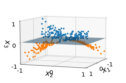
In this example, we explicitly constructed the map $$x\to\phi(x)\quad\textrm{or}\quad(x_1,\;x_2) \to (x_1, \;x_2, \;x_1x_2).$$ Here \(x=(x_1,x_2)\) represents one data sample in the original feature space. \(\phi(x)=(\phi_1,\phi_2,\phi_3)\) represents a data point in the targeting feature space. In this case, we have \(\phi_1(x) = x_1\), \(\phi_2(x) = x_2\), and \(\phi_3(x) = x_1x_2\).
We can get similar results by introducing a kernel function $$K(x,y) \equiv \langle \phi(x), \phi(y) \rangle = x_1y_1 + x_2y_2 + x_1x_2y_1y_2.$$ The operator \(\langle\cdot,\cdot\rangle\) means inner product. Note that we do not need to know the map function \(\phi(x)\) explicitly. We only need the formula of the kernel function. Things are straight forward when we know \(\phi(x)\), but you may wondering how do things work when only \(K(x,y)\) is given?
We are going to work it out step by step. Given a data set of \(n\) samples \(x^{(i)}=(x^{(i)}_1,x^{(i)}_2)\) and the kernel function \(K(x,y)\) defined above (or whatever form you want), we can map an data point \(x^*\) to an \(n\)-dimensional space by $$x^*\to f(x^*) = (f_1,\dots,f_n) \quad \textrm{with} \quad f_i=K(x^*,x^{(i)}).$$ In this example, we can write the mapping in a matrix form with data points as row vectors.
Define $$ \tilde{x}^* = (x^*_1, \;x^*_2, \;x^*_1x^*_2),$$ $$ M = \left( \begin{array}{ccc} x^{(1)}_1 & \cdots & x^{(n)}_1 \\ x^{(1)}_2 & \cdots & x^{(n)}_2 \\ x^{(1)}_1x^{(1)}_2 & \cdots & x^{(n)}_1x^{(n)}_2 \\ \end{array} \right).$$ Then \(f(x^*)=\tilde{x}^*M\). Each row of matrix \(M\) is a vector in the \(n\)-dimensional space. The new feature space defined by the kernel is therefore a subspace spanned by the three row vectors of matrix \(M\).
The map function in this example is relatively simple, so we can recover the original map function directly from the kernel function, i.e. \(\phi(x^*)=\tilde{x}^*\). However, in general we do not need to and won't be able to do such recovery. The main reason is the map function is not unique given one kernel function. In the current example, we can define a new map function by transforming the current vector orthogonally. This won't change the kernel function, but the map function will be different. The orthogonal transformation changes the basis of the new feature space, but not the space itself. We can even define a completely new map function that has the same kernel: \(\phi(x) = (\frac{1}{\sqrt{2}}x_1, \;\frac{1}{\sqrt{2}}x_1, \;x_2, \;x_1x_2)\). Thus, the map function is not unique given a kernel function.
Reproducing Kernel Hilbert Space (RKHS)
As mentioned earlier, we can find many map functions given the same kernel. However, there always exists one unique feature space, which is the reproducing kernel Hilbert space (RKHS); and the map function is given by the kernel. In the simple example above, the subspace spanned by the three \(n\)-dimensional vectors is the RKHS.
The RKHS is the mathematical backup for the kernel trick. It ensures the idea of mapping to a new feature space is always legitimate. In this part, we are going to sketch the proof of the existence of RKHS. The proof can be skipped when applications are the only focuses.
Theorem 1 (Moore-Aronszajn). Let \(X\subseteq\mathbb{R}^n\), and let \(\kappa:X\times X\to\mathbb{R}\) be finitely positive semi-definite. Then there exists a unique RKHS \(\mathcal{H}\subseteq\mathbb{R}^X\) with a unique reproducing kernel \(\kappa\).
Before delving into the proof, we first clarify our notations:
- \(X\): a non-empty set of data
- \(\kappa:X\times X\to\mathbb{R}\): a kernel function
- \(\mathbb{R}^X=\{f|f:X\to\mathbb{R}\}\): a set of all functions from \(X\) to \(\mathbb{R}\)
- \(\mathcal{H}\subseteq\mathbb{R}^X\): an Hilbert space of the new features
- \(\phi:X\to\mathcal{H}\): a feature map
- \(E_x:\mathcal{H}\to\mathbb{R}\): a linear evaluation functional defined by \(f\to f(x)\)
Definition 1 (Finitely Positive Semi-definite Function). \(\kappa\) is finitely positive semi-definite if
- \(\forall\{x_1,\dots,x_m\}\subseteq X\), \(\forall(\alpha_1,\dots,\alpha_m)\in\mathbb{R}^m\), and \(m\) is finite, we have \(\sum_{i,j}\alpha_i\alpha_j\kappa(x_i,x_j)\ge0\).
Definition 1 (Kernel). \(\kappa\) is a kernel if
- \(\exists\phi\), \(\forall x,y\in X\), we have \(\kappa(x,y)=\langle\phi(x),\phi(y)\rangle_{\mathcal{H}}\).
Definition 2 (RKHS). \(\mathcal{H}\) is called a reproducing kernel Hilbert space (RKHS) if
- \(\forall x\in X\), \(E_x\) is bounded and continuous.
Definition 3 (Reproducing Kernel). \(\kappa\) is called a reproducing kernel of \(\mathcal{H}\) if
- \(\forall x\in X\), we have \(\kappa(\cdot,x)\in\mathcal{H}\),
- \(\forall x\in X\), \(\forall f\in\mathcal{H}\), we have \(E_x(f)=\langle f,\kappa(\cdot,x)\rangle\).
Sketch of proof for Theorem 1: Let \(\mathcal{H}_0=\mathrm{span}\{\kappa(\cdot,x)\}_{x\in X}\). Then, we can write any \(f\in\mathcal{H}_0\) as $$f = \sum_{i=1}^m \alpha_i \kappa(\cdot,x_i),$$ for some set of points \(\{x_1,\dots,x_m\}\). Define inner product $$ \langle f, g\rangle_{\mathcal{H}_0} = \sum_{i=1}^m \sum_{j=1}^m \alpha_i \kappa(x_i,x_j) \beta_j,$$ where \(g = \sum_{i=1}^m \beta_i \kappa(\cdot,x_i)\). Add the set of all equivalence classes of Cauchy sequences on \(\mathcal{H}_0\), i.e. make it a Hilbert space. Then \(\mathcal{H}_0\) is the unique RKHS. Suppose \(\mathcal{H}^*_0\) is the topological dual of \(\mathcal{H}_0\). Then \(E_x\in\mathcal{H}^*_0\). From Riesz Representation theorem, \(E_x\) can be represented by a unique \(v_x\in\mathcal{H}_0\), i.e. \(E_x(f)=\langle f,v_x\rangle\) for any \(f\in\mathcal{H}_0\). Therefore, we define \(E_x=\kappa(\cdot,x)\). From definition, \(\kappa\) is a reproducing kernel of \(\mathcal{H}_0\) on \(X\). \(\Box\)
Applications
Now we apply the kernel trick to some linear methods.Kernel PCA
PCA finds directions that have the largest variances of the data. Treat a data set as a matrix \(X\) with \(n\) rows as samples and \(p\) columns as features. Each row \(x_i\) is a row vector representing a sample point. Suppose the data set is centralized, then \(X^TX\) is just the covariance matrix. With singular value decomposition (SVD), we can write \(X=USV^{\dagger}\). Then columns of orthonormal matrix \(V\) are principal components. Given a data point \(x^*\), the transformed data is then \(x^*V\).
To apply the kernel trick, we first need to write \(x^*V\) in forms of inner products. Define \(n\)-by-\(n\) kernel matrix \(K=XX^T\). We can get the orthonormal matrix \(U\) by solving an eigen-problem of \(K\). Each column is an eigenvector ordered by descending eigenvalues \(\lambda_i\). And diagonal elements of \(S\) are just \(\sqrt{\lambda_i}\). Then the transformed data \(\tilde{x}^*\) can be calculated by $$\tilde{x}^*=x^*V = x^*(X^TX)^{-1}X^TUS = x^*X^T (XX^T)^{-1} US$$
Now we want to do PCA after mapping data into a feature space with \(x_i\to\phi(x_i)\). However, we do not know the explicit form of \(\phi\). We only know \(\langle\phi(x_i),\phi(x_j)\rangle=\kappa(x_i,x_j)\). Replace all the inner product by this kernel function, we get $$\tilde{x}^* = X^* K^{-1} U S = X^* U S^{-1}.$$ Here elements of kernel matrix \(K\) and the \(n\)-dimensional row vector \(X^*\) are defined by $$ K_{ij} = \kappa(x_i,x_j), \quad X^*_i=\kappa(x^*,x_i).$$ Note that we used \(K=USS^TU^{\dagger}\) in the last step. Since only diagonal elements of \(S\) are non-zero, the inverse of \(S\) is by inversing all non-zero elements.
Our calculation is based on the assumption that the data set is centralized. However, it is not guaranteed that data in the new feature space satisfies this assumption. Suppose \(\phi_c=\frac{1}{n}\sum_{i=1}^n\phi(x_i)\) is the center of data in the new feature space. Then we should have new $$ \tilde{K}_{ij} = \langle\phi(x_i)-\phi_c,\phi(x_j)-\phi_c\rangle, \quad \tilde{X}^*_{i} = \langle\phi(x^*)-\phi_c,\phi(x_i)-\phi_c\rangle.$$ After simplification, we get $$ \tilde{K} = HKH, \quad \tilde{X}^* = X^* - \bar{K}.$$ Here \(H=I-\frac{1}{n}\mathbb{1}_{n\times n}\) is a projection matrix that centralize rows (or columns) when applied to the right (or left) of a matrix. \(\bar{K}\) is row means of kernel matrix \(K\). Note that we eliminated two constant terms in \(\tilde{X}^*\), because they give zero when multiplied by \(US^{-1}\). It can be easily checked that a row vector with all elements as one is a left eigenvector of matrix \(US^{-1}\) with eigenvalue zero.
Kernel regression
Simple linear regression is to estimate the best \(\beta\) that minimizes the mean square error of a linear prediction \(Y=X\beta\). We consider the case when \(L_2\) regularization is added, i.e. ridge regression with cost function \(L_{\lambda}=||Y-X\beta||^2_2+\lambda||\beta||^2_2\). Estimation of \(\beta\) is then $$\hat{\beta} = (X^TX+\lambda I)^{-1} X^T Y = X^T(XX^T+\lambda I)^{-1} Y.$$ Similarly, we define kernel matrix \(K\) and the \(n\)-dimensional row vector \(X^*\) with elements $$ K_{ij} = \kappa(x_i,x_j), \quad X^*_i=\kappa(x^*,x_i).$$ Then the predicted value of data point \(x^*\) is $$ \hat{y}^* = X^* (K+\lambda I)^{-1} Y.$$
References
- Course PHY598 (Spring2018): Statistical Data Analysis and Stochastic Processes in Physics - by Prof. Jun S. Song.
- Arthur Gretton, Introduction to RKHS, and some simple kernel algorithms pdf)
Comments