Notes on Market

This is a introduction of limear market models based on the course I took in 2017 fall. There are mainly two parts in this post: linear markets and Lemke algorithm for solving linear markets numerically.

Fisher Linear Market

We work to earn money; and we use money to buy what we need. Most of the time the things we need are affordable such as foods, groceries, etc. On the other hand, there are luxury brands that only targets rich people. Have you ever though of what decides prices of all these things? In 1891, Irving Fisher proposed a simple solvable market model in his Ph.D. thesis. In this section, we will formulate this model mathematically following him; and we will describe a numerical algorithm for solving this model in a later section.

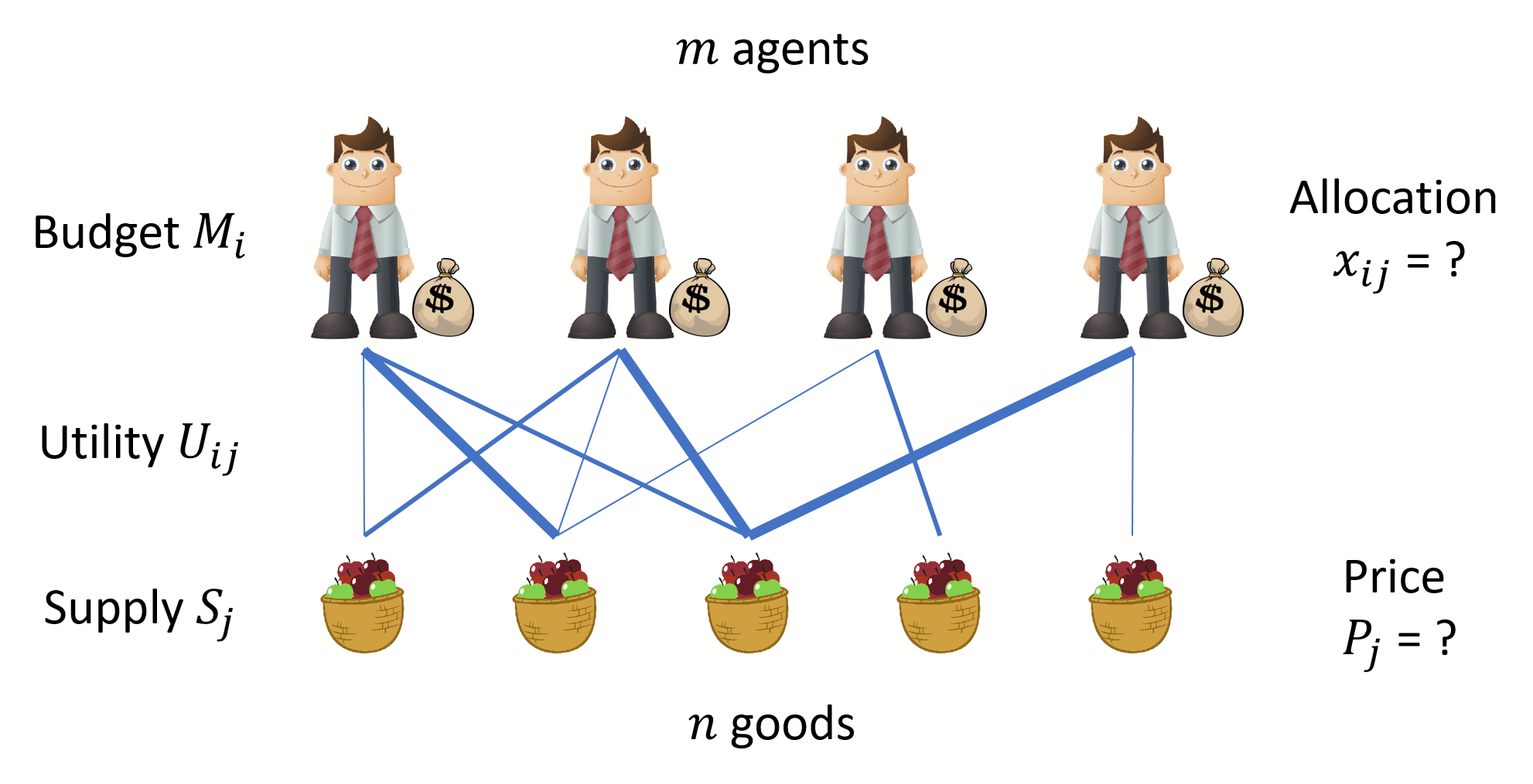
A Fisher market describes a simplified real market which is solvable. Suppose there are \(m\) agents and \(n\) types of divisible goods in a market. As shown in the above cartoon, each agent wants to buy some goods (preferences over different goods are indicated by the width of the lines). However, agents have limited budgets \(M_i\) and numbers of goods \(S_j\) are not infinite. All agents want to maximize their total satisfactory within their budgets. Suppose agent \(i\) bought a boundle of goods \(x_i=\{x_{i1},\dots,x_{in}\}\). His satisfactory over this boundle is indicated by a utility function \(U_i(x_i)\). To make life easier, linear utility functions are used, i.e. \(U_i(x_i) = \sum_{j=1}^n U_{ij}x_j\).

Now we have a full description of the Fisher market: $$\textrm{Fisher}\{M_i, U_{ij}, S_j\}$$

• \(M_i\): budget of each agent \(i\) with \(m\) agents in total.
• \(U_{ij}\): utility function of agent \(i\) over good \(j\).
• \(S_j\): units of divisible good \(j\) with \(n\) kinds of goods in total.

The problem is to find the best \(\{x_{ij},P_j\}\) that maximizes utility functions of all agents. We say the market reaches equilibrium when it clears, i.e. all agents reaches their budgets and all goods are sold. Now we can state the problem as an optimization problem $$\begin{split} \max\sum_{j=1}^n & U_{ij} x_{ij}\quad\forall i\quad\textrm{with constrains}\\ \sum_{j=1}^n & P_{j} x_{ij} = M_i\\ \sum_{i=1}^m & x_{ij} = S_j \\ & P_j>0 \\ & x_{ij}\ge0 \end{split}$$

Exchange Market

It turns out that Fisher linear market is a special case of a more general market model: exchange market. In exchange market, no money is used. Every agent comes with some goods; and they exchange goods directly. This is exactly what people did when money was not invented.

We formulate exchange market as the following. $$\textrm{Exchange}\{W_{ij}, U_{ij}\}$$

• \(W_{ij}\): agent \(i\) has \(W_{ij}\) units of good \(j\).
• \(U_{ij}\): utility function of agent \(i\) over good \(j\).

Note that there is redundant information in this formulation. We can always change the unit of goods and rescale \(U_{ij}\) accordingly. We set \(\sum_i W_{ij}=1\), i.e. measure goods in units of total number of goods \(S_j=\sum_{i} W_{ij}\), Then \(U_{ij}\) should be replaced by \(U_{ij}S_j\).

Fisher market can be easily converted to exchange market. If we treat market as an additional agent and money as an additional good, then Fisher market becomes exchange market automatically. What if we do not want to change the number of agents nor goods? We can still do it. Note that the budget \(M_i\) of each agent indicates his/her buying ability. We can first distribute goods according to the agents' buying abilities discarding their utility functions. This is a fair way to distribute goods. Though the agents may not be satisfied with what they get, they do not lose their buying abilities. After this fair distribution, money becomes useless. All agents can get what they want by exchanging goods directly with each other. Mathematically, it is the same as setting $$ W_{ij} = \frac{M_i}{\sum_i M_i} S_j $$

Similar with the Fisher linear market, the exchange market also has equilibrium \(\{x_{ij}, P_{ij}\}\), which is a solution of $$\begin{split} \max \sum_{j=1}^n & U_{ij} x_{ij}\quad\forall i\quad\textrm{with constrains}\\ \sum_{j=1}^n & P_{j} x_{ij} = \sum_{j=1}^n P_{j} W_{ij} \\ \sum_{i=1}^m & x_{ij} = \sum_{i=1}^m W_{ij} = 1\\ & P_j>0 \\ & x_{ij}\ge0 \end{split}$$ Rescaling the equilibrium price of exchange market has no effects on other values. To get the equilibrium price for Fisher linear market, we only need to rescale the price according to the total money brought to the market, i.e. set \(\sum_j P_j S_j = \sum_i M_i\). Then we can restore the previous conditions with: $$ \sum_i W_{ij} = S_j, \quad\quad \sum_j P_j W_{ij} = M_i .$$

The exchange market is more general than Fisher market. If an exchange market can be converted to Fisher market, it has to satisfy \(W_{ij} = a_ib_j\) (matrix \(W\) is a product of a column vector \(a\) and a row vector \(b\)). There is always equilibrium for Fisher market, but exchange market may not have equilibrium.

Linear Complementarity Problems (LCP)

Before we try to find solutions of the exchange market, we first define linear complementarity problems (LCP). Later we will show that exchange market problems are LCP. As an algorithm for LCP, the Lemke algorithm can be used to solve exchange market problems.

Given a \(n\times n\) matrix \(A\) and a \(n\times 1\) vector \(q\), a LCP is defined by $$ Ay - q \le 0 \;\perp\; y\ge0.$$ Here, \(y\) is the solution vector of length \(n\) we want to find. We use \(\perp\) to indicate the complementarity condition \(y^{T}(Ay-q)=0\). With the inequality constrains, this implies \(y_i (Ay-q)_i=0\) for all \(i\).

When \(q_i\ge0\) for all \(i\), we can easily get the trivial solution \(y_i=0\). Then we can use the Lemke-Howson algorithm (we will describe it later) to find another nontrivial solution. To find all solutions, we can use support enumeration algorithm (we will not talk about this algorithm in this post). When some \(q_i\) are negative, we can still apply the Lemke-Howson algorithm, but with a little modification. We add a non-zero number \(z\) to the original problem. $$ \begin{split} Ay-&z-q \le 0 \;\perp\; y\ge0\\ & \quad z\ge0 \end{split}$$ Then a trivial solution is \(z=\infty\), \(y_i=0\). Start from this trivial solution, we can use the Lemke-Howson algorith to find a solution with \(z=0\). Lemke algorithm implements this idea and solves the problem.

Lemke-Howson algorithm

The conditions \(Ay\le q\) and \(y_i\ge0\) forms a convex polyhedron in the \(n\) dimensional space. Assume the polyhedron is bounded (polytope), otherwise the algorithm may not find a solution. We label conditions \(Ay\le q\) from 1 to \(n\), and the complementary conditions \(y\ge0\) from 1' to \(n\)'. Since a vertex is determined by at least \(n\) equalities, we label vertices of the polytope with labels of tight inequalities. Then each vertex has a label (\(l_1,\dots,l_n\)), where \(l_i \in \{1,\dots,n,1',\dots,n'\}\). The solutions are then vertices with labels including all numbers from 1 to \(n\) (ignore whether it has prime or not).

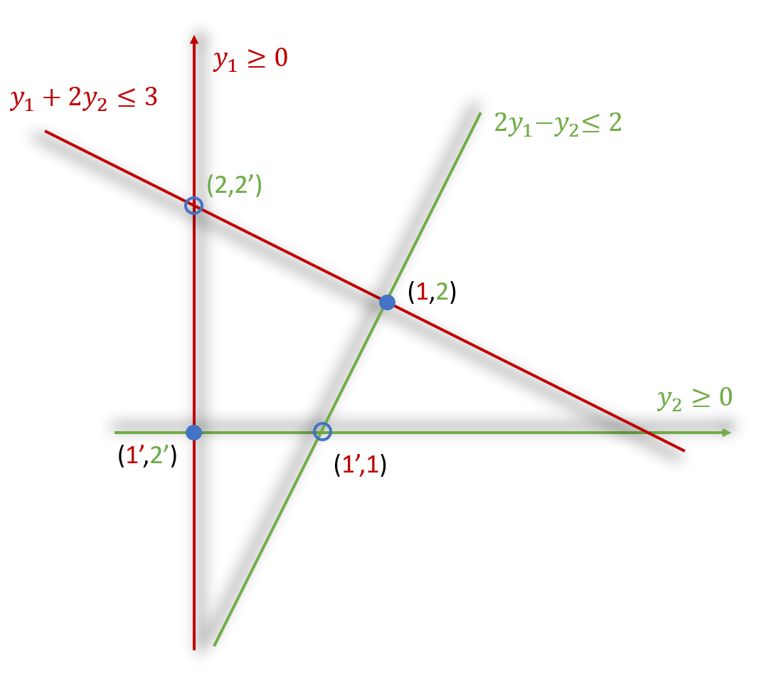
For example, we take \(n=2\) and choose conditions $$\begin{split} & (1)\quad y_1 + 2y_2 \le 3 \;\perp\; y_1 \ge0 \\ & (2)\quad 2y_1 - y_2 \le 2 \;\perp\; y_2 \ge0 \end{split}$$ The corresponding polytope is shown in the figure below. Lines with the same color are complementary conditions. The shades of a line indicate the half plane satisfying the inequality. Vertices are highlighted and associated with labels. Solid dots are solutions while circles are not.

Lemke-Howson algorithm is guaranteed to find one non-trivial solution. Start from the trivial solution \(y_i=0\) and choose a label \(k\in\{1,\dots,n\}\).

1. set initial vertex as \(y=(0,\dots,0)\), which has label (\(1',\dots,n'\))
2. relax equation \(k'\), so we can move along the edge defined by \(y_j=0\) for \(j\neq k\) and \(y_k\ge0\)
3. find the other vertex \(y'\) of the edge.
4. find index \(j\) of the newly satisfied equation; then vertex \(y'\) has label \((1',\dots,(k-1)',j,(k+1)',\dots,n')\)
5. while label of vertex \(y'\) has duplicating index \(j\)
   • relax equation \(j'\) and find the label of next vertex \(y'\).
6. \(y'\) is a solution of the LCP

The algorithm creates a path from initial trivial solution to another solution. In the above example, if we choose \(k=1\), then the path is \((1',2')\to(2,2')\to(1,2)\). It is easy to show that the vertices within a path has no \(k\) or \(k'\) in their labels. The two edge vertices of a path have labels that include all numbers. Therefore only the two edge vertices are solutions of the LCP. When \(k\) is given then the path is unique. There cannot be crossings in a path. Since every vertices can be accessed at most once, the worst running time of this algorithm scales as the number of vertices.

Lemke algorithm

Lemke-Howson algorithm only works when \(q\) is non-negative. When \(q\) has negative elements, we cannot choose \(y_i=0\) as the starting solution. But we can modify the problem by adding a positive number \(z\) to \(q\), so that \(q_i+z\) are all non-negative.

$$ \begin{split} Ay-&z-q \le 0 \;\perp\; y\ge0\\ & \quad z\ge0 \end{split}$$ As mentioned before, \(y_i=0\) and \(z=\infty\) is a solution of this new problem. In fact, all points on \(y_i=0\) and \(z\ge\max(-q_i)\) are solutions. These solutions form a ray, called the primary ray.

Similar with the Lemke-Howson algorithm, we start from a trial solution vertex then move along edges of polyhedron to find the solution we want. In the Lemke algorithm, the starting vertex satisfies \(y_i=0\) and \(z=\max(-q_i)\). Then the condition \((Ay-z-q)_i=0\) automatically satisfies. Therefore, the starting vertex has label \((1',\dots,i',i,(i+1)',\dots,n')\). Note that the space dimension is \(n+1\) instead of \(n\), so we always have two same numbers in a label if \(z\neq0\). We want a solution with \(z=0\), so the solution vertex is again labeled with no repeating numbers.

In both the Lemke-Howson and the Lemke algorithms, we find solutions by moving along edges of the polyhedron defined by the constrains. In the Lemke-Howson algorithm, only starting and ending vertices satisfy complementary conditions. However, in the Lemke algorithm all passing edges and vertices are solutions of the new problem with \(z\) included. Only the vertex with \(z=0\) is a solution of the original LCP problem.

There are two potential problems of the Lemke algorithm: rays and degeneracies. It is not guaranteed that we will always find a vertex when we move along an edge. These edges stretching to infinity are secondary rays. For market problems, no secondary rays exist. It is possible that the number of tight conditions is larger than the space dimension. In such case the path direction is not uniquely determined. We choose the direction that minimizes \(z\) most.

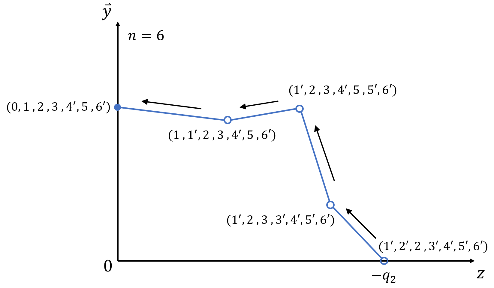
Consider an example with \(n=6\). The illustration is shown in the above plot. Since it is not easy to plot a high dimensional space on a 2D plane, we use one direction for values of \(z\) and the other for the vector space \(\{y_1,\dots,y_n\}\). The vertices are associated with labels. Arrows indicate the direction of the path.

The running time of the Lemke algorithm is linear in number of vertices. It can be easily proven by the fact that each vertex can only be accessed at most once along the path. The actual running time is in fact faster for most cases.

Codes

In this section, we describe the algorithms in detail and post the python codes. Following notations in previous sections, we define functions Lemke_Howson and Lemke.

def Lemke_Howson(A, q, k=0):
    """
        This solves the LCP problem: Ay<=q, y>=0, y(Ay-q)=0.
        All elements of q are non-negative.
        input:  A:  numpy array of dimension (n,n)
                q:  numpy array of dimension (n,)
                k:  integer from 0 to n-1, default to be 0
        output: y:  numpy array of dimension (n,)
                    return None if encounter a ray
    """

    n = A.shape[0]

    # Write all linear constraints with one matrix
    M = np.vstack([A, -np.identity(n)])
    b = np.hstack([q, np.zeros(n)])

    # initial trivial vertex
    y = np.zeros(n)
    ii = n+k

    y, ii = FindNextVertex(M, b, y, ii)
    if ii==-1:
        return None
    count = 1    # store the number of pivotings 
    while ii!=k and ii!=n+k:    # while label k is not achieved
        count += 1
        if ii<n:
            y, ii = FindNextVertex(M, b, y, ii+n)
        else:
            y, ii = FindNextVertex(M, b, y, ii-n)
        if ii==-1:
            return None
    return y

def Lemke(A, q):
    """
        This solves the LCP problem: Ay<=q, y>=0, y(Ay-q)=0.
        input:  A:  numpy array of dimension (n,n)
                q:  numpy array of dimension (n,) 
                k:  integer from 0 to n-1, default to be 0
        output: y:  numpy array of dimension (n,)
                    return None if encounter a ray
    """
    n = A.shape[0]

    # add positive number z to the problem Ay-z<=q
    # Write all linear constraints with one matrix
    M = np.vstack([np.hstack([A, -np.ones([n,1])]), -np.identity(n+1)])
    b = np.hstack([q, np.zeros(n+1)])

    # starting vertex
    y = np.zeros(n+1)
    ii = np.argmin(q)
    y[n] = np.max(-q[ii], 0)

    count = 0    # store the number of pivotings 
    while y[n]>epsilon:    # while z is not zero
        count += 1
        if ii<n:
            y, ii = FindNextVertex(M, b, y, ii+n)
        else:
            y, ii = FindNextVertex(M, b, y, ii-n)
        if ii==-1:
            return None
    return y[:n]

The key step is to find the next vertex, which is defined in function FindNextVertex. Before we come to this function, we review a few things in geometry. Suppose \(x\) represents a point in space \(\mathbb{R}^n\).

• The linear function \(w^Tx=a\) defines a plane. Vector \(w\) gives the norm direction of the plane. It points out of the area \(w^Tx\le a\)
• The intercept of \(n\) non-parallel planes is a point in the space. Given a non-singular \(n\times n\) matrix \(M\), inequality \(Mx\le q\) defines a vertex of a polyhedron. The directions of edges from this vertex are columns of \(-M^{-1}\)

Start from a vertex \(v\) and an edge directing to \(d\), we want to find the other vertex. Suppose we know that a plane \(w^Tx=a\) cut the edge. Then it must satisfy \(d^Tw>0\). The new vertex must be \(v+\beta d\) for some \(\beta\). Since it is a point on the plane, we can solve \(\beta\) from \(w^T(v+\beta d)=a\). Following is the code to find the next vertex.

def FindNextVertex(M, b, v, k):
    """
        Find the next vertex of polyhedron Mv<=b from the current vertex v 
        by relaxing tight constrain with index k
        input:  M:  numpy array of dimension (m, n)
                b:  numpy array of dimension (m,)
                v:  numpy array of dimension (n,)
                k:  integer from 0 to n-1
        output: v:  numpy array of dimension (n,)
                k:  integer from 0 to n-1
    """

    # index of tight inequalities
    tight = np.argwhere( np.abs(M.dot(v)-b) < epsilon ).ravel()

    # find direction of the edge
    dire = -np.linalg.inv(M[tight,:])[:, list(tight).index(k)]

    betamin = np.inf
    for i, w in enumerate(M):
        alpha = np.dot(w, dire)
        if (not i in tight) and (alpha>0):
            beta = (b[i]-np.dot(w,v)) / alpha
            if beta<betamin:
                betamin = beta
                k = i
    if betamin is np.inf:
        return v, -1
    if verbose:
        print("start from", v, "end at", v+betamin*dire)
    v = v+betamin*dire
    return v, k

LCP Formulation of the Exchange Market

Now we know how to solve a LCP using the Lemke algorithm. However, neither the Fisher linear market or the exchange market is a LCP. We need complementary conditions and transform equality constrains into inequalities.

We first define auxiliary parameters $$ \begin{split} \frac{1}{\lambda_i} & = \max_k\frac{U_{ik}}{P_k} \\ f_{ij} & = x_{ij} P_j \\ \tilde{P}_j & = P_j-1 \end{split}$$ Here \(\lambda_i\) is the minimum money agent \(i\) need to pay for one unit of satisfactory. \(f_{ij}\) is the money agent \(i\) paid for good \(j\). It is defined to remove the non-linearity. We define \(\tilde{P}_j\), so that constraint \(P_j>0\) can be written as \(\tilde{P}_j\ge0\).

To reach maximum satisfactory for each agent we notice that an agent \(i\) only buy goods whose value matches \(\lambda_i\). Therefore, we get our first complementary constraint $$ \lambda_iU_{ij} - (\tilde{P}_j+1) \le 0 \;\perp\; f_{ij} \ge 0$$

The market clear constraints can be written with \(\{f_{ij},\tilde{P}_j\}\) as $$\begin{split} & \sum_i^m f_{ij} \le (\tilde{P}_j+1)\\ & \sum_j^n f_{ij} \ge \sum_j^n W_{ij}(\tilde{P}_j+1) \end{split}$$ With \(\sum_i W_{ij}=1\) we can easily see that both inequalities are strict. We can add redundant complementarily constraints with these inequalities.

Since we have \(-\sum_j^n W_{ij}\) as part of \(q\) vector, we add auxiliary parameter \(z\) to the problem. Note that \(z\) is only added to all the inequalities. Now, we have the LCP formulation of market problems $$\begin{split} - \tilde{P}_j + U_{ij}\lambda_i \le 1 & \;\perp\; f_{ij} \ge 0 \\ \sum_i^m f_{ij} - \tilde{P}_j \le 1 & \;\perp\; \tilde{P}_j \ge 0 \\ -\sum_j^n f_{ij} + \sum_j^n W_{ij} \tilde{P}_j - z \le -\sum_j^n W_{ij} & \;\perp\; \lambda_i \ge 0 \end{split}$$ This problem has no secondary ray. Thus the Lemke algorithm converges to the market equilibrium.

Now we try to solve a simple Fisher linear market: $$M=\left(\begin{array}[cc] &10 \\ 10 \\ \end{array}\right),\quad U=\left(\begin{array}[cc] &1 & 0 \\ 2 & 1 \\ \end{array}\right),\quad S =\left(\begin{array}[cc] &1 & 1 \\ \end{array}\right)$$ By running the program (link), we get the solution at the 5th vertex. $$x=\left(\begin{array}[cc] &3/4 & 0 \\ 1/4 & 1 \\ \end{array}\right),\quad P =\left(\begin{array}[cc] &40/3 & 20/3 \\ \end{array}\right)$$

References

1. Course IE598 (Fall2017): Games, Markets, and Mathematical Programming - by Jugal Garg. (Course website)
2. William Brainard and Herbert Scarf. How to compute equilibrium prices in 1891. Cowles Foundation Discussion Paper, 1270, 2000. (pdf)
3. A COMPLEMENTARY PIVOT ALGORITHM FOR MARKET EQUILIBRIUM UNDER SEPARABLE, PIECEWISE-LINEAR CONCAVE UTILITIES. (pdf)
4. All python codes are converted into colored format with hilite