Mean Field Theory and Boltzmann Machine

In classical statistics, we treat a physical system as an ensemble of elementary particles. For example, a magnet can be described by spins from iron ions. The probability distribution of states of the system is given by Boltzmann distribution $$ P(\mathbf{X}) = \frac{1}{Z} e^{-\beta E(\mathbf{X})}. $$ Here we use vector \(\mathbf{X}\) to denote states. \(E(\mathbf{X})\) is energy of given states. \(Z=\sum_{\mathbf{X}} e^{-\beta E(\mathbf{X})} \) is a normalization factor and \(\beta=1/T\) with \(T\) as temperature.

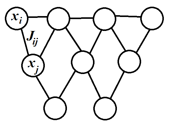
It turns out that there are deep connections between spin systems in physics and undirected graphical models in computer science. In the language of computer science and statistics, the vector \(\mathbf{X}\) is considered as a vector of random variables. The Boltzmann distribution gives their joint distribution. Such kind of network is called Boltzmann machine (wiki). It is a type of Markov random field, in which a variable is conditionally independent of all other variables given its neighbors (Local Markov property). Particularly, for Boltzmann machine we have \(x_i\in\{\pm1\}\) and energy $$ E = -\sum_{i,j} J_{ij} x_i x_j - \sum_i h_i x_i $$ It makes Boltzmann machine identical to classical Ising model in external fields.

When we try to calculate expectation values, the full joint distribution is intractable. The number of summation terms increases exponentially with the number of particles (or random variables). This strictly restricts the size of system to be small. However, in both physics and computer science we want to be able to deal with much larger systems. As physicists, we use approximations in such situations. We use tractable distributions to approximate the exact distribution and then do calculations.

In the following, we will try to find the approximated distributions of Boltzmann distribution. We first introduce naïve mean field theory, then improve it by including corrections. The relationship between TAP, Bethe approximation and Belief propagation will also be discussed. Since I am a physicist, I will describe from a physics perspective of view. The counterpart from computer science will be put in the shaded box.

Gibbs free energy

We first note that Boltzmann distribution is the distribution that minimizes Gibbs free energy (Details of the proof can be found in appendix A). Gibbs free energy is defined by $$ G = U - TS = \sum_{\mathbf{X}} P(\mathbf{X}) E(\mathbf{X}) + T \sum_{\mathbf{X}} P (\mathbf{X})\ln P(\mathbf{X})$$ Here, \(U\) is expected energy and \(S\) is entropy of the distribution.

Now the problem of finding best tractable distributions to approximate Boltzmann distribution becomes finding tractable distributions \(Q(\mathbf{X})\) to minimize Gibbs free energy.

Since Boltzmann distribution \(P(\mathbf{X})\) is minimum, whatever distribution \(Q(\mathbf{X})\) we find must have larger or equal Gibbs free energy. The minimum Gibbs free energy is just Helmholtz free energy $$ F = -T \ln Z $$ Therefore, we get the inequality $$-T\ln Z \le \sum_{\mathbf{X}} Q(\mathbf{X})E(\mathbf{X}) -T\sum_{\mathbf{X}}- Q(\mathbf{X})\ln Q(\mathbf{X})$$ We can reach the same conclusion using the non-negative property of Kullback-Leibler divergence.

Naïve mean field approximation

The simplest assumption on \(Q(\mathbf{X})\) would be completely independence. Assume all the spins are in an effective potential and no interactions between spins. Energy function is of form \(E=-\sum_jV(x_j)\). Thus, we can decompose Boltzmann distribution as $$ Q(\mathbf{X}) = \frac{1}{Z} e^{\beta\sum_jV(x_j)} = \prod_j\frac{1}{Z_j} e^{\beta V(x_j)} \equiv \prod_j Q_j(x_j)$$

Define \(m_i=\sum_{x_i}Q(x_i)x_i\) as magnetization. In the case when \(x_i\in\{\pm 1\}\), we can get the probability from magnetization \(Q(x_i=\pm1)=(1\pm m_i)/2\). If we can solve for \(m_i\), the distribution \(Q(\mathbf{X})\) is solved. The Gibbs free energy under mean field assumption becomes $$ \begin{split} G_{\mathrm{MF}} = & - \sum_{(i,j)} J_{ij} m_i m_j - \sum_i h_i m_i \\ & + T \sum_i \left[ \frac{1+m_i}{2} \ln \left(\frac{1+m_i}{2}\right) + \frac{1-m_i}{2} \ln \left(\frac{1-m_i}{2}\right)\right] \end{split}$$ We want to minimize Gibbs free energy. By setting first derivative with respect to \(m_i\) as zero and second derivative no less than zero, we get $$ m_i = \tanh \left(\frac{h_i+\sum_j J_{ij}m_j}{T}\right)$$ which is not too difficult to solve numerically.

Correcting naïve mean field

Bethe approximation

We made a strong assumption in naïve mean field theory that all spins are in effective single-particle potentials. Now we weaken the assumption by including two-particle potentials. Then the distribution is of form $$ Q(\mathbf{X}) = \prod_i Q_i^{-(q_i-1)} (x_i) \prod_{i,j} Q_{ij}(x_i,x_j) $$ where \(q_i\) is number of spins connected with spin \(i\), i.e. non-zero number of \(J_{ij}\) given \(i\). Here, all the distributions are marginal distributions. The factor \(q_i-1\) is a correction for over counting. Note that this distribution is exact for Bethe lattice, which has the same topology with a rooted tree.

The Gibbs free energy under this approximation becomes $$ \begin{split} G_{\mathrm{Bethe}} =& - \sum_{i,j} Q_{ij}(x_i,x_j) J_{ij} x_i x_j - \sum_i Q_i(x_i)h_i x_i \\ & + T \sum_i (1-q_i) Q(x_i)\ln Q(x_i) + T \sum_{i,j} Q_{ij}(x_i,x_j)\ln Q_{ij}(x_i,x_j) \end{split}$$

Minimizing this Gibbs free energy is again a constraint minimization problem, since all \(Q_i(x_i)\) and \(Q_{ij}(x_i,x_j)\) should be probability distributions. After adding Lagrange multipliers, we can get equations for \(Q_i(x_i)\) and \(Q_{ij}(x_i.x_j)\) $$ Q_i(x_i) = \frac{e^{-E_i(x_i)/T}}{Z_i} \exp\left[\frac{\sum_j \lambda_{ji}(x_i)}{T(1-q_i)}\right] $$ $$ Q_{ij}(x_i,x_j) = \frac{e^{-E_{ij}(x_i,x_j)/T}}{Z_{ij}} \exp\left[\frac{\lambda_{ji}(x_i)+ \lambda_{ij}(x_j)}{T}\right] $$ where \(E_i(x_i)=-h_i x_i\) and \(E_{ij}(x_i,x_j)=-J_{ij}x_ix_j-h_i x_i-h_j x_j\). The Lagrange multipliers \(\lambda_{ij}\) can be solved by applying the marginalization condition \(Q_i(x_i) =\sum_{x_j} Q_{ij}(x_i,x_j)\). We get $$ \lambda_{ij}(x_j) = T \ln \prod_{k\in N(j)} M_{kj}(x_j) $$ and $$ M_{ij}(x_j) \propto \sum_{x_i} e^{-[E_ij(x_i,x_j)-E_j(x_j)]/T}\prod_{k\in N(i)} M_{ki}(x_i)$$ Here, \(N(i)=\{j|J_{ij}\ne0 \textrm{ or } J_{ji}\ne0\}\) is a set of spins neighboring spin \(i\). These equations can be solved iteratively. Note that the marginal distributions are just belief functions in belief propagation algorithm and \(M_ij\) are messages.

Plefka's expansion

Now we try to get the approximate distributions from another direction. We do not restrict the form of approximate distributions. We add constraints to the exact distribution, then minimize Gibbs free energy with constraints. It is not that straight forward as previous methods, but we will reach the same results.

Given a vector \(\mathbf{m}\) with elements \(m_i\), we add constraints to the probability distribution \(Q(\mathbf{X})\) $$ \langle \mathbf{X} \rangle_Q = \mathbf{m} $$ The minimization problem with constraints is again solved by using Lagrange multiplier. We want to minimize $$ G(\mathbf{m})= \langle E(\mathbf{X})\rangle_Q - TS[Q] - T\sum_i \lambda_i (\langle x_i \rangle_Q - m_i) $$ The last term can be combined into the energy term. Therefore, the minimizing distribution is just $$ Q_{\mathbf{m}}(\mathbf{X}) = \frac{1}{Z} e^{-\beta E(\mathbf{X})+\sum_i \lambda_i (x_i-m_i)} $$ where \(\beta=1/T\). Plug in \(Q_{\mathbf{m}}(\mathbf{X})\), we get our Gibbs free energy $$ \beta G(\mathbf{m})= -\ln \sum_{\mathbf{X}} e^{-\beta E(\mathbf{X})+\sum_i \lambda_i (x_i-m_i)} $$

Expand \(G(\mathbf{m})\) near \(\beta=0\) and replace \(\lambda_i\) calculated from constraints, we get the terms untill the second order of \(\beta\) $$ \begin{split} & \beta G_0(\mathbf{m}) = \sum_i \left[ \frac{1+m_i}{2} \ln \left(\frac{1+m_i}{2}\right) + \frac{1-m_i}{2} \ln \left(\frac{1-m_i}{2}\right)\right] \\ & \beta G_1(\mathbf{m}) = - \sum_{i,j} J_{ij} m_i m_j \\ & \beta G_2(\mathbf{m}) = - \frac{1}{2} \sum_{i,j} J_{ij}^2(1-m_i^2)(1-m_j^2) \end{split}$$ All these terms add up to the Thouless-Anderson-Palmer (TAP) expansion $$ \begin{split} G_{\mathrm{TAP}} = & - \sum_{(i,j)} J_{ij} m_i m_j - \frac{1}{2T} \sum_{(i,j)} J_{ij}^2(1-m_i^2)(1-m_j^2) \\ & + T \sum_i \left[ \frac{1+m_i}{2} \ln \left(\frac{1+m_i}{2}\right) + \frac{1-m_i}{2} \ln \left(\frac{1-m_i}{2}\right)\right] \end{split}$$

This Gibbs free energy is claimed to be exact for Sherrington-Kirpatrick (SK) model. It is an infinite-ranged Ising spin class model with zero external field. The interaction matrix is symmetric and each element \(J_{ij}\) is chosen from normal distribution with variance \(J_0/N\).

TAP equation for SK model is $$ \langle S_i\rangle =\tanh \left(\sum_j J_{ij}\langle S_j\rangle - J_0 (1-q) \langle S_i\rangle + h_i \right) $$ where \(q=\frac{1}{N} \sum_j (1-\langle S_j\rangle^2)\).

Note that TAP approach and belief propagation give rise to the same equations in general.

Appendix

A: Boltzmann distribution minimizes Gibbs free energy

Suppose \(P\) is a functional of \(\{x_i\}\). We want to minimize $$G = \sum_{\{x_i\}} P E + T \sum_{\{x_i\}} P \ln P$$ under constraint \(h = \sum_{\{x_i\}} P -1\). Using Lagrange multiplier, we transform the problem to be minimizing \(\tilde{G}=G+\lambda h\) without constraints. At minimum, the variant of \(G\) under variant of \(P\) should be zero $$\frac{\delta\tilde{G}}{\delta P} = E + T (\ln P +1) + \lambda = 0 $$ The derivative with respect to \(\lambda\) gives back us the original constraint $$ \frac{\partial\tilde{G}}{\partial\lambda} = \sum_{\{x_i\}} P - 1 = 0$$ Solve the two equations above, we get $$ P = \frac{1}{Z} e^{-E/T} $$ which is Boltzmann distribution. \(\lambda\) is chosen to satisfy the normalization condition and is absorbed into \(Z\).

References

1. Opper, Manfred, and David Saad, eds. Advanced mean field methods: Theory and practice. MIT press, 2001